Capstone 49 — Graphs, Ontologies & GraphRAG

A plain-English guide to graphs, knowledge graphs, ontologies, graph neural networks, and GraphRAG with formulas and PyTorch examples.

← Full AI Course · ← AI Agents · Next: Frontier Watch →

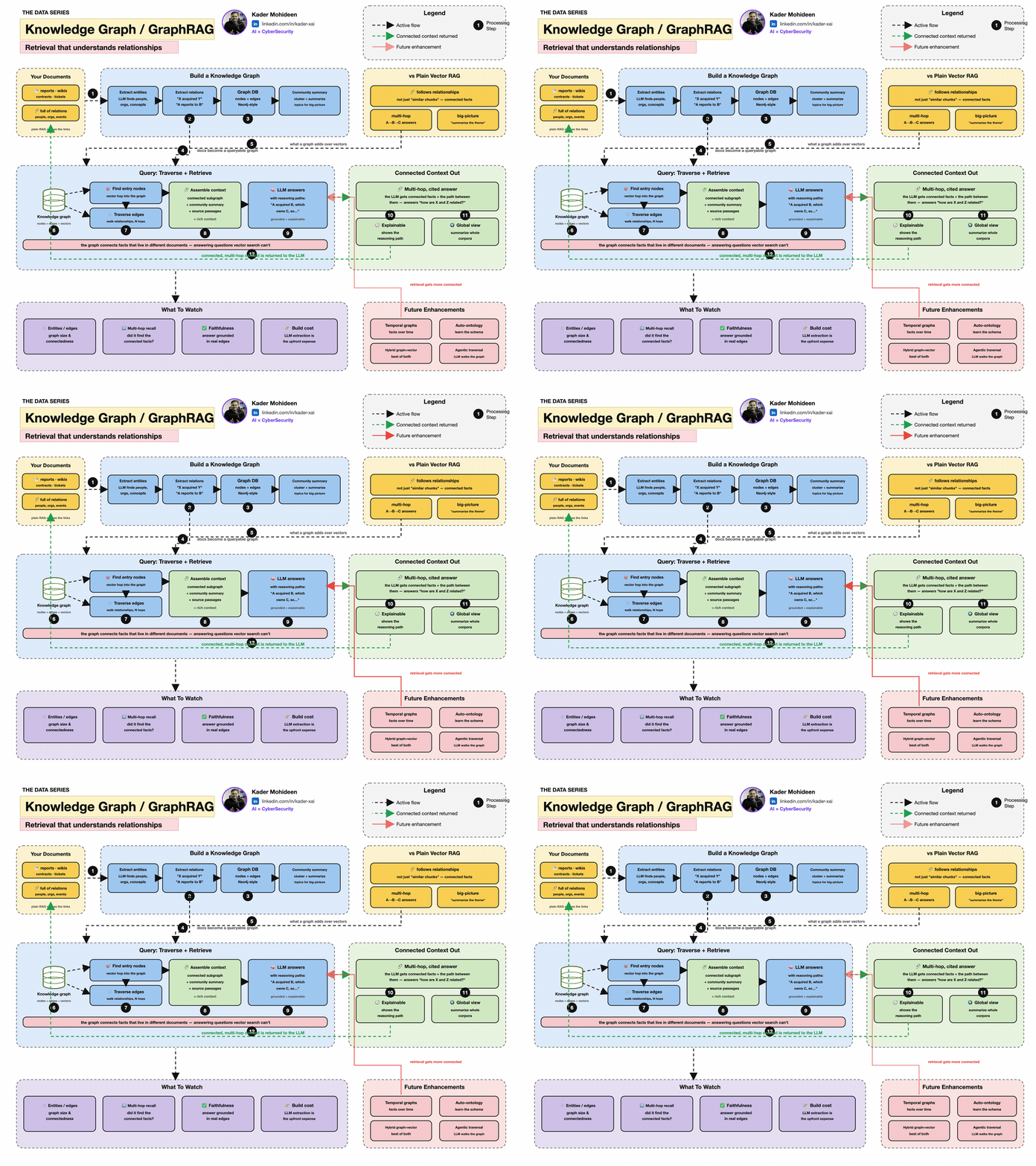
A table is excellent when every row has the same shape. A graph is better when the connections are part of the meaning: people know people, devices talk to services, hotels sit in districts, and documents mention organizations.

This capstone separates four related ideas that are often blended together.

Idea	What it provides	Simplest mental picture
Graph	Nodes and edges	Things connected to things
Knowledge graph	Meaningful entities and relationships	Facts stored as a network
Ontology	Shared types, properties, and rules	The grammar of the knowledge
GraphRAG	Graph-based context for an LLM	Retrieve connected evidence before answering

1. Start with a triple

A knowledge graph can be built from simple subject–predicate–object triples:

(Hotel_A, located_in, Riyadh)
(Hotel_A, has_control, CCTV)
(CCTV, mitigates, Physical_Intrusion)
(Physical_Intrusion, is_a, Security_Risk)

The nodes are entities such as Hotel_A and CCTV. The labeled edges—located_in, has_control, and mitigates—state what the relationships mean.

An ontology adds a shared contract:

Hotel is a type of Property.
has_control connects a Property to a Security_Control.
every CCTV is a Security_Control.
mitigates connects a control to a risk.

Now a reasoner can infer that Hotel_A is a Property and that its CCTV is a security control, even if those two facts were not written directly.

Graph = connections. Knowledge graph = meaningful facts. Ontology = agreed vocabulary and rules. You can have a graph without an ontology, but an ontology makes independently created data easier to combine and reason over.

2. Graphs as matrices

For three nodes, an adjacency matrix \(A\) records which pairs are connected:

\[ A=\begin{bmatrix} 0 & 1 & 1\\ 1 & 0 & 0\\ 1 & 0 & 0 \end{bmatrix} \]

Row 1 says node 1 connects to nodes 2 and 3. A zero means no direct edge. This matrix representation lets standard linear algebra operate on a graph.

import torch

A = torch.tensor([
    [0., 1., 1.],
    [1., 0., 0.],
    [1., 0., 0.]
])

degree = A.sum(dim=1)
print(degree)  # tensor([2., 1., 1.])

The degree is simply the number of neighbors. In directed or weighted graphs the same idea extends to incoming, outgoing, or weighted connections.

3. A graph neural network in one formula

A Graph Convolutional Network lets each node update its representation from its neighbors:

\[H^{(l+1)}=\sigma\left(\hat D^{-1/2}\hat A\hat D^{-1/2}H^{(l)}W^{(l)}\right)\]

Read it from right to left:

\(H^{(l)}\) contains the current feature vector for every node.
\(W^{(l)}\) learns which feature combinations matter.
\(\hat A=A+I\) adds a self-connection so each node keeps its own information.
\(\hat D^{-1/2}\) normalizes for nodes with many neighbors.
\(\sigma\) adds a non-linear activation.

The same layer written directly in PyTorch:

import torch

# 3 nodes, each with 2 input features
H = torch.tensor([
    [1.0, 0.2],
    [0.1, 1.0],
    [0.8, 0.4]
])
A = torch.tensor([
    [0., 1., 1.],
    [1., 0., 0.],
    [1., 0., 0.]
])
W = torch.tensor([
    [0.7, -0.2],
    [0.3,  0.8]
])

A_hat = A + torch.eye(A.shape[0])
degree = A_hat.sum(dim=1)
D_inv_sqrt = torch.diag(degree.pow(-0.5))
A_norm = D_inv_sqrt @ A_hat @ D_inv_sqrt

H_next = torch.relu(A_norm @ H @ W)
print(H_next)

This is message passing: transform each node’s information, send it along the edges, aggregate what arrives, and update the node.

4. Ontologies in RDF and OWL

The Semantic Web stack provides standard ways to express graph facts and schemas:

RDF represents triples.
RDFS adds basic classes, properties, domains, and ranges.
OWL adds richer logical statements and constraints.
SPARQL queries RDF graphs.

A tiny example in Turtle syntax:

@prefix ex: <https://example.org/> .
@prefix rdfs: <http://www.w3.org/2000/01/rdf-schema#> .

ex:Hotel rdfs:subClassOf ex:Property .
ex:CCTV rdfs:subClassOf ex:SecurityControl .
ex:Hotel_A a ex:Hotel ;
    ex:hasControl ex:Camera_7 .
ex:Camera_7 a ex:CCTV .

Because Hotel is a subclass of Property, a reasoner can infer:

Hotel_A is a Property

The strength of an ontology is not that it adds more text. It adds shared meaning that software can check.

5. Embeddings and symbolic meaning are complementary

An embedding maps an item into a learned vector. It is good at similarity: “these two passages feel related.” An ontology is good at explicit meaning and rules: “a hotel is a property, and every property must have an owner.”

Embeddings	Ontologies
Fuzzy similarity	Explicit semantics
Learned from data	Designed or curated
Tolerant of wording differences	Supports rules and consistency checks
Can be difficult to explain	Human-readable relationships

Modern systems combine them: vectors retrieve semantically similar evidence; graphs connect entities; ontologies constrain the vocabulary; an LLM turns the retrieved evidence into an answer.

6. What GraphRAG changes

Basic RAG usually retrieves text chunks whose vectors are close to the question. This is strong for local questions, but it can miss answers that require connecting distant facts.

GraphRAG first extracts entities, relationships, and claims, builds communities in the graph, and prepares summaries. At question time it can retrieve around a specific entity or reason over broader community summaries. Microsoft’s current GraphRAG overview describes this indexing pipeline, and the query documentation separates local, global, DRIFT, and basic search modes.

Documents→Entities + relations→Communities→Evidence→Answer

GraphRAG is not automatically better for every question. Its indexing can cost more, extracted graphs can contain mistakes, and simple vector search may be faster and sufficient for direct fact lookup.

7. A hybrid retrieval score

A practical retriever can combine vector similarity with graph distance:

\[\text{score}(d,q)=\alpha\,\cos(e_d,e_q)+(1-\alpha)\frac{1}{1+\operatorname{dist}_{G}(d,q)}\]

In words: reward semantic similarity between document and question embeddings, then add a graph bonus for evidence close to the relevant entity.

import torch
import torch.nn.functional as F

query = torch.tensor([[0.9, 0.1, 0.4]])
documents = torch.tensor([
    [0.8, 0.2, 0.5],
    [0.2, 0.9, 0.1],
    [0.6, 0.1, 0.7]
])
graph_distance = torch.tensor([1., 0., 3.])

semantic = F.cosine_similarity(documents, query.expand_as(documents))
graph_bonus = 1 / (1 + graph_distance)
alpha = 0.75
score = alpha * semantic + (1 - alpha) * graph_bonus

print(score)
print("best document:", score.argmax().item())

The weights must be tuned on real questions. A beautiful formula is not a substitute for evaluation.

8. Common failure modes

Entity duplication — “Kader Mohideen,” “Kader M.,” and “Kader” become three nodes.
Wrong edge direction — controls is stored as controlled_by.
Schema drift — different teams invent overlapping relationship names.
Hallucinated relationships — the extraction model adds a plausible but unsupported edge.
Stale facts — a correct relationship changes over time.
Graph explosion — everything connects to everything, so retrieval becomes noise.
False authority — the graph looks structured, so users assume every fact is true.

Preserve provenance for every extracted claim: source document, location, extraction time, and confidence. The graph should make evidence easier to inspect, not hide it.

9. When to use what

Need	Good starting point
Find passages similar to a question	Vector RAG
Answer questions about relationships	Knowledge graph
Enforce shared types and business rules	Ontology
Learn from network structure	Graph neural network
Connect distant facts across a corpus	GraphRAG
Small, clean, relational dataset	SQL may be enough

Continue the course: deepen the pieces in Linear Algebra, Probabilistic Graphical Models, Knowledge Representation & Reasoning, Graph Machine Learning, and Information Retrieval.

← AI Agents · Course map · Next capstone: Frontier Watch →